Abstract
A linear relationship for Reynolds number and flow speed in an Osborn Reynold's apparatus found a turbulent flow speed of $U = 18,73 \,\frac{\textrm{cm}}{\textrm{s}}$ and a corresponding Reynold's number of $Re = 2243$, which was consisted with the expected transition region between laminar and turbulent flow. Reversible flow was unsuccessfully demonstrated with the Taylor-Couette demonstration due to the lower viscosity of the shampoo fluid used.
Theory
Because fluid flow is so mathematically complicated, idealizations are often necessary to describe a system. Sometimes, this takes the form of ideal flow, where viscous effects are assumed to be small. However, when viscous forces are significant, and therefore cannot be ignored, we can sometimes use the Laminar flow approximation.
The key parameter in characterizing flow as laminar or not laminar is the Reynold's number, defined as[1]: $$\begin{align} Re\equiv\frac{\rho uL}{\mu} \tag{1} \end{align}$$ $u$ represents the velocity of the fluid, $L$ represents the diameter of the apparatus' pipe, $\rho$ represents the fluid density, and $\mu$ represents the dynamic viscosity of the fluid. These last two terms are often combined, forming a new term called the dynamic viscosity $\nu\equiv\frac{\mu}{\rho}$. Note that the Reynold's number is a dimensionless quantity. For $Re<2000$, fluid flow is characterized as laminar, and for $Re>3000$, the flow is characterized as turbulent [2]. The region between $2000 < Re < 3000$ is considered the transition region between laminar and turbulent flow since the definition of turbulent flow requires a level of observational intuition and choice. Laminar flow is convenient, because it allows us to work with linear differential equations.
The Osborne Reynold's apparatus is used to demonstrate the difference between laminar and turbulent flow. This experiment used the apparatus to calculate Reynold's number at various flow speeds, and attempted to locate the transition point between laminar and turbulent flow. In practice, the transition does not occur at a single "point", rather there is a spectrum between laminar and turbulent flow.
The Taylor-Couette apparatus demonstrates the reversible nature of laminar flow. To ensure the flow is laminar, a highly viscous fluid must be used, and the apparatus must be turned slowly and carefully.
Proceadure
Osborne Reynold's Apparatus
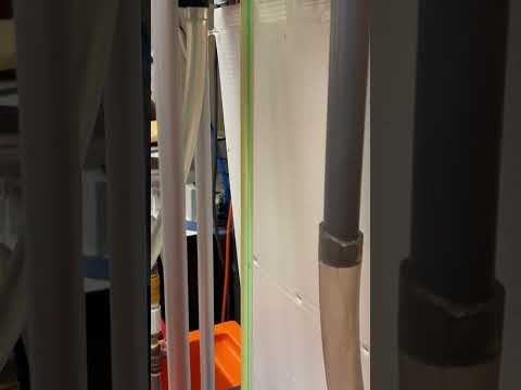
The Osborne Reynold's apparatus contains a transparent vertical pipe of a fixed diameter, and a pipette placed above the mouth of the pipe. The pipette was opened to let a small amount of dye flow through the pipe. At the bottom of the pipe was a valve, which could be turned to adjust the flow rate $Q$: $$ Q = \frac{\textrm{Flask Volume }V}{\textrm{Time to fill Volume }t} $$
To collect data, the time taken for the water flowing out the bottom of the apparatus to fill a 300 mL beaker was measured. This, in combination with the cross sectional area of the pipe $A$, gave us the flow speed $U$, which was then used to calculate Reynold's number: $$ U \,[\tfrac{\textrm{m}}{\textrm{s}}] = \frac{Q \,[\textrm{Litres / s}]}{A \,[\textrm{m}^2]} $$
Taylor-Couette Flow
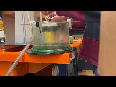
The Taylor-Couette demo consists of two concentric cylinders with a viscous fluid between them (in our case, shampoo). Some dye was inserted into the fluid, and the innermost cylinder was turned clockwise seven times, causing the dye to be stirred. The flow was then reversed, i.e. the cylinder was turned clockwise seven times, causing the dye to be un-stirred.
Data & Observations
Pipe diameter, $d = 0.012\,\mathrm{m}$
Water density, $\rho=1000\,\mathrm{kg/m^3}$
Dynamic viscosity of water, $\mu=1.00\cdot10^{-3}\,\mathrm{kg/m/s}$
Measuring the flow rate $Q$ and converting to $U$ for given $A$ from $d$, the Reynold's numbers for each respective $U$ were calculated using Eq.(1) and are illustrated in Table 1 and Fig.(1):
| Time, $t$ ($s$) | Volume, $V$ ($mL$) | Reynold's Number, $Re$ | Flow Speed, $U$ ($m/s$) |
|---|---|---|---|
| 154.43 | 300 | 205.7 | 0.0172 |
| 46.57 | 300 | 255.8 | 0.0214 |
| 124.19 | 300 | 628.6 | 0.0525 |
| 23.89 | 300 | 682.1 | 0.0570 |
| 14.16 | 300 | 1089.4 | 0.0910 |
| 50.54 | 300 | 1227.0 | 0.1025 |
| 23.82 | 300 | 1329.7 | 0.1110 |
| 29.16 | 300 | 1333.6 | 0.1114 |
| 15.77 | 300 | 1520.0 | 0.1269 |
| 25.89 | 300 | 1913.7 | 0.1598 |
| 20.90 | 300 | 2014.4 | 0.1682 |
| 16.60 | 300 | 2243.5 | 0.1873 |
| 12.68 | 300 | 2505.3 | 0.2092 |
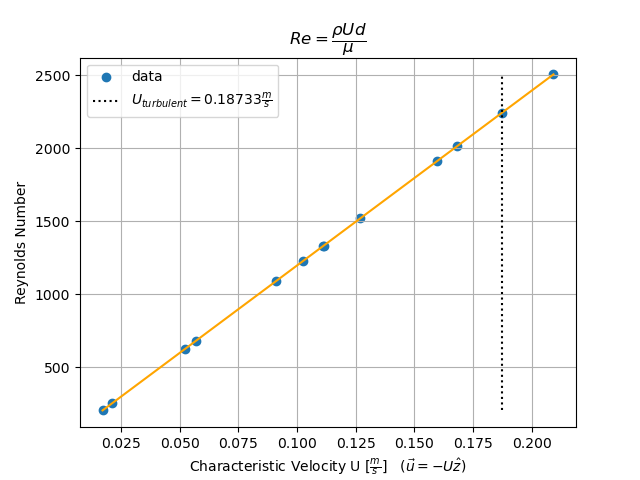
Notes: The flow appeared to be laminar for most of the data points. Since there is no clear delineation between laminar and turbulent flow, we used our judgment and came up with a cutoff point.
Links to videos:
- Laminar Flow 1: https://www.youtube.com/shorts/TEzE60RD-I8
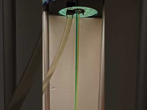
- Laminar Flow 2: https://youtube.com/shorts/YqWjUm5XM9g
- Reversible Flow: https://www.youtube.com/watch?v=LzJbvO8tlJE
Discussion & Tips for the Next Class
The relationship between $Re$ and $U$ is linear as expected by Eq.(1) and consistent with turbulent $Re$ values given by Kundu et al. (2025). We achieved a transition to turbulent flow at $U = 18,73 \,\frac{\textrm{cm}}{\textrm{s}}$ and a Reynold's number of $Re = 2243$.
The primary source of systematic uncertainty on these values arise from the measurement of the volume of water filled in the flask, the accuracy of the timing to fill this volume, which incorporates a systematic bias to measurements, and the measurement of $d$. The latter was estimated for the inner-diameter of the downward pipe with a ruler, though a caliper measurement with the bottom hose removed may achieve more accurate results for $d$. While consistent with the expected $Re$ at turbulent transition, another analysis of decreasing flow from turbulent to laminar could be done to observe how close the transition point is from the reverse procedure to that found here.
Time permitting, performing several runs of both approaches of the turbulent region will give a statistical analysis of the transition region $Re \in (2000,\,3000)$. The results would describe whether whether one side of the transition region is favoured separately by one approach or if both favour the same side or none.
The Taylor-Couette demonstration did not work as intended to demonstrate reversible flow. Since the Reynold's number was too high, this suggests either the apparatus was turned too quickly, or the fluid was not viscous enough to limit diffusivity of the dye. Using fresh, clear, and unused corn starch or glycerine would help achieve higher viscosities, and a more stable and fixed apparatus for the spin mount would also help achieve the ideal conditions to replicate the Taylor-Coutte demonstration.
References
[1]: Kundu, P. K., Cohen, I. M., Dowling, D. R., & Capecelatro, J. (2025). 4.11 Dimensionless forms of the equations and dynamic similarity. In Fluid Mechanics (7th ed., pp. 124–130). Chapter Section, Academic Press.
[2]: Kundu, P. K., Cohen, I. M., Dowling, D. R., & Capecelatro, J. (2025). 7.1 Laminar Flow Introduction & 7.2 Exact solutions for steady state incompressible viscous flow. In Fluid Mechanics (7th ed., pp. 223–230). Chapter Section, Academic Press.
Appendix A: Code for values and plots
import numpy as np
import matplotlib.pyplot as plt
rho = 1000 # kg / m^3
mu = 1.002e-3 # kg / m / s
d = 0.012 # m
flask_vol = 300 # mL
Area = np.pi * d**2 / 4
time = np.array([154.43, 46.57, 124.19, 23.89, 14.16, 50.54, 23.82,
                 29.16, 15.77, 25.89, 20.9, 16.60, 12.68]) # seconds
# print(time)
# print(np.sort(time))
Q = np.sort(np.sort(flask_vol / time)) # ml / s
U = Q / 1e6 / Area # m / s (fluid speed)
Rey = rho * U * d / mu # Reynolds number
for i in range(len(Rey)):
    print(f't:  {time[i]:.2f}')
    print(f'Re: {Rey[i]:.1f}')
    print(f'U:  {U[i]:.4f}')
    print()
t:  154.43
Re: 205.7
U:  0.0172

t:  46.57
Re: 255.8
U:  0.0214

t:  124.19
Re: 628.6
U:  0.0525

t:  23.89
Re: 682.1
U:  0.0570

t:  14.16
Re: 1089.4
U:  0.0910

t:  50.54
Re: 1227.0
U:  0.1025

t:  23.82
Re: 1329.7
U:  0.1110

t:  29.16
Re: 1333.6
U:  0.1114

t:  15.77
Re: 1520.0
U:  0.1269

t:  25.89
Re: 1913.7
U:  0.1598

t:  20.90
Re: 2014.4
U:  0.1682

t:  16.60
Re: 2243.5
U:  0.1873

t:  12.68
Re: 2505.3
U:  0.2092
# turbulent velocity
i_turb = np.where(time == 16.60)
U_turb = U[i_turb][0]
Rey_turb = Rey[i_turb][0]
print(f'Turbuent velocity first seen: U = {U_turb:.5f} m / s')
print(f'Corresponding Reynolds Number:    {Rey_turb:.0f}')
Turbuent velocity first seen: U = 0.18733 m / s
Corresponding Reynolds Number:    2243
fig, ax = plt.subplots()
ax.scatter(U, Rey, label = 'data')
ax.plot(U, Rey, c = 'orange')
ax.plot(U_turb * np.ones(len(U)), Rey, ls = ':', c = 'k',
        label = r'$U_{turbulent} = $' + f'{U_turb:.5f}' + r'$\frac{m}{s}$')
ax.set_xlabel(r'Characteristic Velocity U $[\frac{m}{s}]$   ($\vec{u} = -U\hat{z}$)')
ax.set_ylabel('Reynolds Number')
ax.set_title(r'$Re = \dfrac{\rho U d}{\mu}$')
ax.legend()
ax.grid()
# fig.savefig('PHYS426_Laminar_Flow_Plot.png', format = 'png')
