::: center Gravity Waves
Lukas Booy, Everett Schwarz
University of Victoria, Victoria, British Columbia, Canada
Submitted April 6, 2026 :::

Shallow Water Waves {#shallow-water-waves .unnumbered}

This experiment was designed to investigate wave propagation in shallow water flumes, resonance behavior in a large tidal tank, and particle paths using ink and different wave heights. Firstly, two small flumes of equal length ($l = 30.5 ~\rm cm$) were first filled to different water depths (2.5 cm and 4.6 cm) and one side of each was lifted to an equal height of 1.2 cm. The flumes were then released simultaneously to generate waves propagating back and forth along the channel. When released, a timer was commenced to measure the time taken for ten complete reflections along the flume length, with an experimental wave speed measured to be:

\[c_{\rm exp} = \frac{10L}{t_{10}}\]

Where $L$ is the flume length and $t_{10}$ was the time for ten reflections. This was repeated for multiple heights, ascending from 2.5 cm to 3.4 cm for the first tank and descending from 4.6 cm to 3.4 cm for the second, and compared to the theoretical shallow water wave speed.

Shallow water waves are defined as having a surface displacement much less than the weir depth, or $\eta \ll d$. Another way to define this limit is the wavelength being much greater than the water depth, $\lambda \gg d$. Using the governing equations of the flat-bottom case ($\partial_xd = 0$):

\[\begin{equation*} \rm{x-mom:} ~\partial_t u \approx -g \partial_x \eta, \quad~\rm{cont.:} ~\partial_t \eta \approx -d \partial_x u \end{equation*}\]

combining these gives the wave equation:

\[\begin{equation*} \partial_{tt} \eta - gd \partial_{xx}\eta = 0 \end{equation*}\]

with a wavespeed

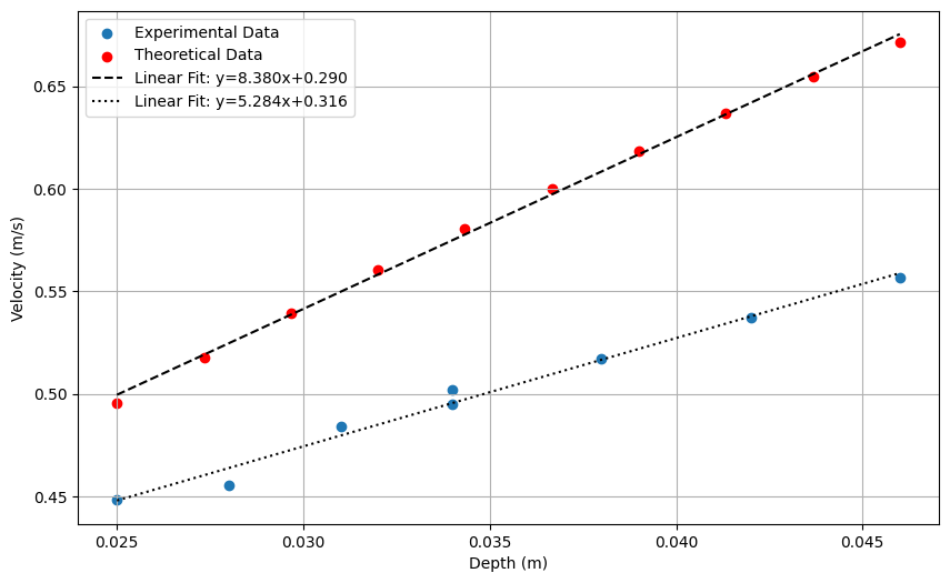
\[\begin{equation*} c = c_g =c_p = \pm \sqrt{gd} \end{equation*}\]

After the first experiment, with the different-depth flumes, the experimental propagation speed $c_{\exp}$ was compared to that of the depth-dependent theoretical value of $c_{\rm theo} = \sqrt{gd}$ The results are given in table 1 below, and visualized in figure 1.

::: {#tab:velocity_depth}

Depth [m] $c_{\rm exp}$ [m/s] $c_{\rm theo}$ [m/s]

————- ———————– ————————

0.025 0.449 0.495

0.028 0.455 0.525

0.031 0.484 0.551

0.034 0.495 0.578

0.034 0.502 0.578

0.038 0.517 0.611

0.042 0.537 0.642

0.046 0.557 0.672

Comparison of Experimental and Theoretical Velocities vs Depth :::

{#fig:placeholder width=”80%”}

From the graph we can see that there is a non-linear loss of velocity between the theoretical and experimental values. The loss increases proportional to velocity and thus indicates the presence of bottom friction in the flume tank.

Resonant Frequencies {#resonant-frequencies .unnumbered}

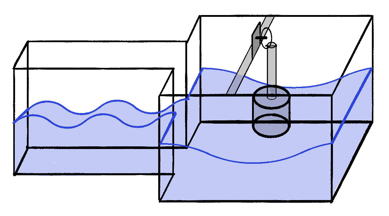
Following the small flume experiments, attention was turned to the large tidal tank. The tank was filled to an initial depth of approximately 9 cm before the session to allow temperature and turbulent conditions to settle. A tidemaker (plunger) was set up near the end of the deep reservoir, and was powered by a voltage range of $6~V\to17~V$, increasing the angular speed of the plunger (set up shown in figure 2). During the tuning of the voltage, the repetitions per second and the corresponding amplitudes of each frequency were measured until there was no noticeable change in the amplitude difference. The depth of the tank was then set to 8 cm and finally 7 cm, and the procedure was repeated for these surface heights.

{#fig:placeholder width=”80%”}

A rotating plunger, with rotational period $T$, generates waves/tides at a frequency of $f = 1/T$. The finite length of the tank supports the standing wave modes, the resonance of which occur every half wavelength: $\lambda_n = 2L/n, ~(n=1,2,3,…)$, or wavenumber $k_n = 2\pi /\lambda_n = n\pi /L$. Combining with the dispersion relation at the shallow water limit:

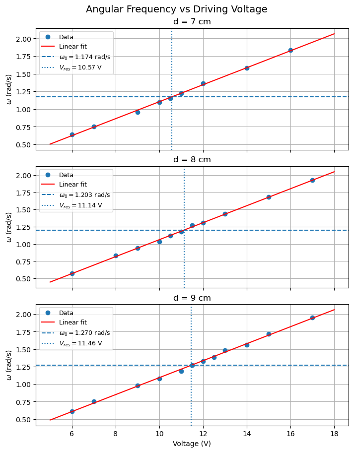
\[\omega_n^2 = gk_n \tanh(k_n d) \rightarrow \omega_n = \sqrt{gd} \cdot k_n\]

Therefore, each harmonic occurs at a frequency

\[f_n = \frac{\omega_n}{2\pi} = \frac{n}{2L}\sqrt{gd}\]

If the forcing frequency matches a natural frequency, $f \approx f_n$, then resonance may occur.

The frequency data collected for a range of voltages is displayed below for each of the depths, with the expected resonant frequency and corresponding voltage indicated by dashed/dotted lines.

The amplitudes over a range of angular speed were plotted and fitted to a theoretical driven/damped harmonic oscillator function of the form:

\[A(\omega)= \frac{A_0}{\sqrt{(\omega-\omega_0)^2 + (2\gamma\omega)^2}}\]

With the results shown in Figure 4.

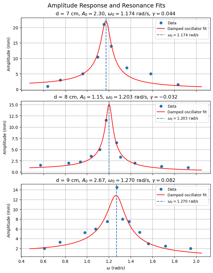
The results showed that both the resonant frequency and corresponding driving voltage increased with water depth, in agreement with the theoretical prediction of $f_n \propto \sqrt{d}$. The resonance curves are well described by a driven/damped harmonic oscillator model, with sinusoidal driving generated by the plunger mechanism and the overall damping caused by bottom friction and reflections off the apparatus walls. Discrepancies arise due to the limitations of the idealized harmonic oscillator model, which don’t fully describe the molecular level interactions which fluids experience during boundary layer interactions.

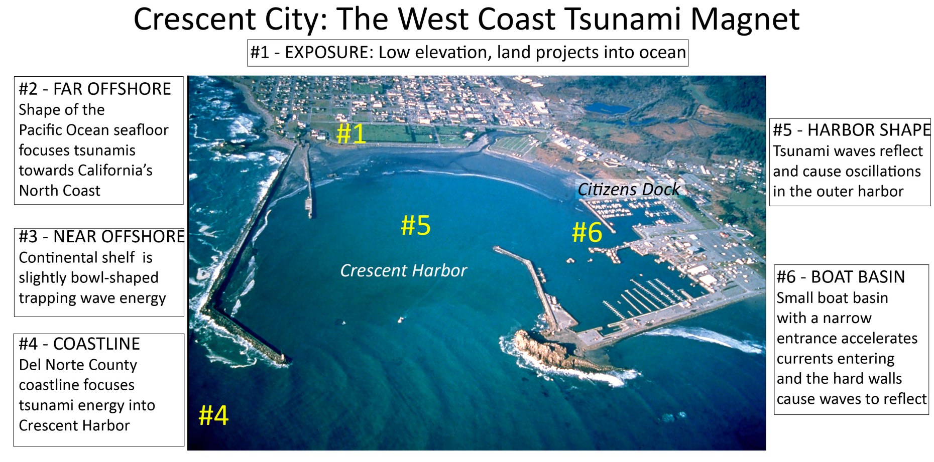
Wave structure is a very important consideration for coastal and ocean engineering, since resonance can significantly increase the amplitude of surface waves in confined basins. In particular, harbors, inlets, and marinas may have increased wave activity when the incoming wave forcing has a frequency close to one of the basin’s normal modes. Under these conditions, even a relatively small external disturbance can produce extremely large oscillations in both water level and current speeds. This can lead to destruction or damage to boats, increased strain on docks, and unsafe operating conditions for workers near said harbors.

One example, seen below, is the Crescent City harbor (in California, USA), which has experienced tsunami conditions 31 times since a tide gauge was established in 1933 $^{[1]}$. This is due to the bathymetry of the sea floor surrounding the coastal city causing a focusing of tsunamis into the port via a ridge off the coast dubbed the Mendocino Fracture Zone $^{[1]}$. When the large waves hit deeper water, their speed increases and could have a chance of having a normal mode frequency of the harbor, causing the waves to increase even more in amplitude.

Deep vs. Shallow Water Waves {#deep-vs.-shallow-water-waves .unnumbered}

Finally, the deep water condition ($\lambda \gg d$ or $kd \gg 1$) was simulated by creating small wave packets by rapidly moving a paddle at the mouth of the tidal flume channel. This was done after injecting ink along a vertical profile to better visualize the particle paths at different water depths for different wave extremes.

In the deep water limit, the dispersion relation becomes $\omega^2 = gk$ (because $\tanh (kd) \to 1$) and the phase and group speed are:

\[c_p = \frac{\omega}{k} = \sqrt{\frac{g}{k}} = \sqrt{\frac{g \lambda}{2\pi}}\] \[c_g = \partial_k\omega = \frac12 \sqrt{\frac{g}{k}} = \frac12 c_p\]

Thus, when visualizing wave packets traveling in deep water, the waves will travel through the packet at approximately twice the speed of the group. This means that crests outrun the front of the packet and emerge from the back of the packet.

From Khundu & Cohen (2008), waves are classified as deep-water waves if the depth is only $28 \%$ more than the wavelength ($kd > 1.75$ or $d > 0.28\lambda$) $^{[3]}$. Particle orbits in such waves travel in ellipses with semiminor and semimajor axes nearly equal to $ae^{kz}$, or circles with a decay scale described by the particle excursion equations below (defined as $u = \partial_t \xi, ~w = \partial_t \zeta$):

\[\xi = -ae^{kz_0} \sin (kx_0 - \omega t), ~\zeta = ae^{kz_0} \cos(kx_0 - \omega t)\]

In the shallow water approximation ($kd \ll 1$), Khundu & Cohen (2008) once again state that surface waves are shallow-water if the water depth is less than 7% of the wavelength ($d < 0.07 \lambda$) $^{[3]}$. In this regime, particle excursion equations become:

\[\xi = -\frac{a}{kd} \sin (kx - \omega t), ~\zeta = a\left(1+ \frac zd\right) \cos (kx - \omega t)\]

These are thin ellipses with a depth-independent semimajor axis and a linearly decreasing semiminor axis (zero at the bottom).

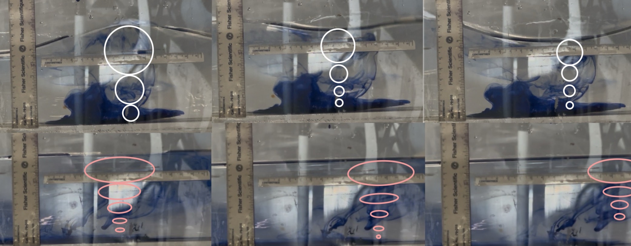
The effects of simulated deep and shallow water waves were visualized using ink and different wave heights. Longer waves were observed to make the ink move uniformly, whereas shorter, higher amplitude waves moved the ink in large circles near the surface of the water and induced minimal movement near the bottom of the tank. Heat diffusion may have caused some extra movement since the water was not of perfectly uniform density. These effects were simulated below, with the “shallow water” particle paths drawn with red ellipses and the “deep water” with white circles.

For Next Time... {#for-next-time… .unnumbered}

- A long, constant depth wave tank would make for easier visualizations and differentiation between shallow and deep water characteristics.

- When placing ink on the bottom, allow for proper vertical diffusion for easy visualization of the particle excursions.

- Put more effective reflection damping at the end of the tidal flume channel to minimize dispersive interference.

References {#references .unnumbered}

[1] Dengler, L., Uslu, B., Barberopoulou, A., Borrero, J., & Synolakis, C. (2008). The vulnerability of Crescent City, California, to tsunamis generated by earthquakes in the Kuril Islands region of the Northwestern Pacific. Seismological Research Letters, 79(5), 608–619. https://doi.org/10.1785/gssrl.79.5.608

[2] Dengler, L. (2025, August 9). Lori Dengler | When it comes to tsunamis, Crescent City is a special place. Times-Standard. https://www.times-standard.com/2025/08/09/lori-dengler-when-it-comes-to-tsunamis-crescent-city-is-a-special-place/

[3] Kundu, P. K., & Cohen, I. M. (2010). Fluid Mechanics. Academic Press.