Usage guide

Installation

pip install mpl-direct-layout

Registering the engine

Import mpl_direct_layout once before creating figures. The import patches matplotlib.figure.Figure.set_layout_engine() so that the string 'direct' is recognised:

import mpl_direct_layout
import matplotlib.pyplot as plt

After that, use layout='direct' anywhere Matplotlib normally accepts a layout engine name:

fig, axs = plt.subplots(2, 2, layout='direct')

fig = plt.figure(layout='direct')

mpl.rcParams['figure.layout'] = 'direct'

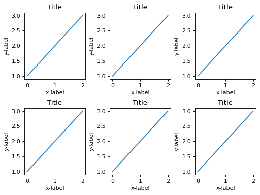
Basic grid

import mpl_direct_layout
import matplotlib.pyplot as plt

fig, axs = plt.subplots(2, 3, layout='direct')
for ax in axs.flat:
    ax.plot([1, 2, 3])
    ax.set_xlabel('x-label')
    ax.set_ylabel('y-label')
    ax.set_title('Title')
plt.show()

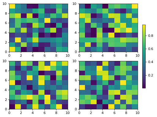
Colorbars

Shared colorbars work in all four locations:

import mpl_direct_layout
import matplotlib.pyplot as plt
import numpy as np

fig, axs = plt.subplots(2, 2, layout='direct')
for ax in axs.flat:
    pcm = ax.pcolormesh(np.random.rand(10, 10))
fig.colorbar(pcm, ax=axs, location='right', shrink=0.6)
plt.show()

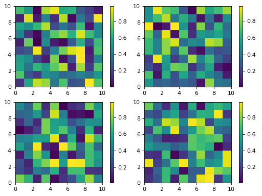
Individual colorbars can be added to each axes:

import mpl_direct_layout
import matplotlib.pyplot as plt
import numpy as np

fig, axs = plt.subplots(2, 2, layout='direct')
for ax in axs.flat:
    pcm = ax.pcolormesh(np.random.rand(10, 10))
    fig.colorbar(pcm, ax=ax, location='right')
plt.show()

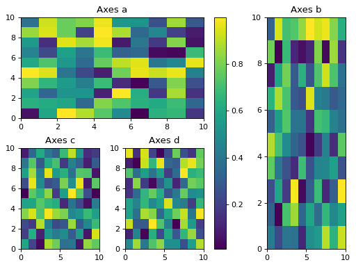
Mosaic layouts

import mpl_direct_layout
import matplotlib.pyplot as plt
import numpy as np

fig = plt.figure(layout='direct')
axd = fig.subplot_mosaic([['a', 'a', 'b'],
                           ['c', 'd', 'b']])
for label, ax in axd.items():
    pcm = ax.pcolormesh(np.random.rand(10, 10))
    ax.set_title(f'Axes {label}')
fig.colorbar(pcm, ax=[axd['a'], axd['c'], axd['d']], location='right')
plt.show()

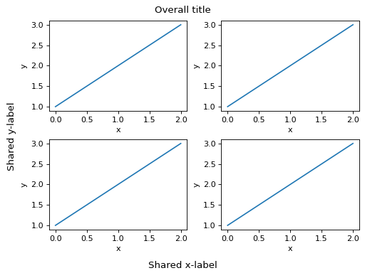
Super-labels

import mpl_direct_layout
import matplotlib.pyplot as plt

fig, axs = plt.subplots(2, 2, layout='direct')
for ax in axs.flat:
    ax.plot([1, 2, 3])
    ax.set_xlabel('x')
    ax.set_ylabel('y')
fig.suptitle('Overall title')
fig.supxlabel('Shared x-label')
fig.supylabel('Shared y-label')
plt.show()

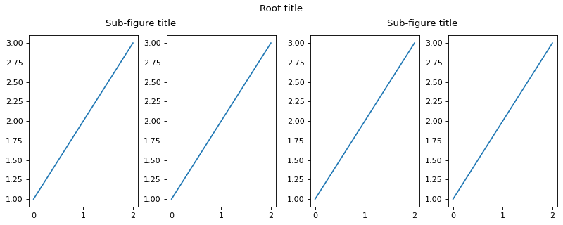
Subfigures

import mpl_direct_layout
import matplotlib.pyplot as plt

fig = plt.figure(layout='direct', figsize=(10, 4))
sfigs = fig.subfigures(1, 2)
for sf in sfigs:
    axs = sf.subplots(1, 2)
    for ax in axs:
        ax.plot([1, 2, 3])
    sf.suptitle('Sub-figure title')
fig.suptitle('Root title')
plt.show()

Tuning parameters

Retrieve the engine with get_layout_engine() and call set():

eng = fig.get_layout_engine()
eng.set(
    h_pad=6/72,        # 6 pt gap between rows (default 3 pt)
    w_pad=6/72,        # 6 pt gap between columns
    left=0.2,          # 0.2" left outer margin
    right=0.1,
    top=0.1,
    bottom=0.15,
    suptitle_pad=0.15, # 0.15" below suptitle
)

All lengths are in inches.

Comparison with constrained_layout

mpl-direct-layout targets the same use-cases as constrained_layout:

Feature	constrained	direct
Regular grids	✓	✓
Spanning / mosaic axes	✓	✓
Colorbars	✓	✓
Shared colorbars	✓	✓
suptitle / supxlabel	✓	✓
Subfigures	✓	✓
Requires kiwisolver	yes	no
`hspace` / `wspace`	✓	✗ (use h_pad)